In [3]:
plt.scatter(X1,Y1,label="F")
plt.scatter(X2,Y2,label="P")
plt.legend()
Out[3]:
<matplotlib.legend.Legend at 0x720bc92e2270>

# 使用するライブラリのimport
import numpy as np
import pandas as pd
import matplotlib.pyplot as plt
%matplotlib inline
# データの生成
np.random.seed(100)
X1 = np.random.normal(7,5,100)
Y1 = np.random.normal(15,5,100)
X2 = np.random.normal(15,5,100)
Y2 = np.random.normal(4,4,100)
plt.scatter(X1,Y1,label="F")
plt.scatter(X2,Y2,label="P")
plt.legend()
<matplotlib.legend.Legend at 0x720bc92e2270>
plt.scatter(X1,Y1,label="F")
plt.scatter(X2,Y2,label="P")
plt.legend()
plt.scatter(7,2,marker="$NEW$",s=500)
<matplotlib.collections.PathCollection at 0x720bc91e20c0>

x1_ave = np.average(X1)
y1_ave = np.average(Y1)

x2_ave = np.average(X2)
y2_ave = np.average(Y2)

plt.scatter(X1,Y1,label="F")
plt.scatter(X2,Y2,label="P")
plt.scatter(x1_ave,y1_ave,marker="*",s=500,color="white",edgecolors="k")
plt.scatter(x2_ave,y2_ave,marker="*",s=500,color="white",edgecolors="k")
plt.scatter(7,2,marker="$NEW$",s=500)
plt.legend()
<matplotlib.legend.Legend at 0x720bc8f395b0>

F_distance = np.sqrt((7 - x1_ave)**2 + (2 - y1_ave)**2)
P_distance =  np.sqrt((7 - x2_ave)**2 + (2 - y2_ave)**2)
print(F_distance,P_distance)
12.659487545459246 8.8583183121659
# 特徴量xと特徴量yをまとめます

F = []

for i,j in zip(X1,Y1):
    F.append(np.array([i,j]))

P = []

for i,j in zip(X2,Y2):
    P.append(np.array([i,j]))
# Fクラスの分割
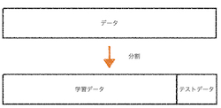
test_F,train_F = F[:20],F[20:]

# Pクラスの分類
test_P,train_P = P[:20],P[20:]
# テストデータのラベルの作成
N = test_F + test_P
L = [0]*20+[1]*20
# それぞれのクラスで平均値を計算

x = 0
y = 0

for i,j in train_F:
    x += i
    y += j

F_ave = np.array([x/80,y/80])

x = 0
y = 0

for i,j in train_P:
    x += i
    y += j

P_ave = np.array([x/80,y/80])
plt.figure()

for i in train_F:
    plt.scatter(i[0],i[1],color="b")

for i in train_P:
    plt.scatter(i[0],i[1],color="r")

plt.scatter(F_ave[0],F_ave[1],marker="*",s=500,color="y",edgecolors="k")
plt.scatter(P_ave[0],P_ave[1],marker="*",s=500,color="y",edgecolors="k")

for i in N:
    plt.scatter(i[0],i[1],color="None",edgecolors="k")

| 本当\自動 | 合格 | 不合格 | |
|---|---|---|---|
| 合格 | a | b | |
| 不合格 | c | d |
この表は列が自動採点、行が本当の合否です。
正確度(Accuracy): 全体の中で正しく判定されている割合(確率) $$\frac{a+d}{a+b+c+d}$$
偽陰性率 (False negative) : 本当は合格しているのに自動採点が不合格と判定する割合(確率) (この値が高いと自動採点の方が「厳しい」と評価できる)
$$\frac{b}{a+b}$$偽陽性率(False positive): 本当は不合格なのに自動採点が合格と判定する割合(確率)(この値が高いと自動採点が「甘い」と評価できる)
$$\frac{c}{c+d}$$再現率(感度、真陽性率、Recall): 本当に合格した人の中で合格者を発見できる割合(確率) $$\frac{a}{a+b}$$
適合率(精度、陽性反応的中度、Precision): 自動採点が合格と判定したときに本当に合格である割合(確率) $$\frac{a}{a+c}$$
特異度(真陰性率、Specificity): 不合格の人に対して、不合格と判定する割合(確率) $$\frac{d}{c+d}$$
# 自動採点システムによる評価を取得

y_pred = []

for i in N:
    f = np.linalg.norm(F_ave - i)
    p = np.linalg.norm(P_ave - i)
    if p < f:
        y_pred.append(1)
    else:
        y_pred.append(0)
print(y_pred)
[0, 0, 1, 0, 0, 0, 0, 0, 0, 0, 0, 0, 0, 1, 0, 0, 0, 0, 0, 0, 1, 1, 0, 0, 1, 1, 1, 1, 1, 1, 1, 1, 1, 0, 1, 1, 1, 1, 1, 1]
print(L)
[0, 0, 0, 0, 0, 0, 0, 0, 0, 0, 0, 0, 0, 0, 0, 0, 0, 0, 0, 0, 1, 1, 1, 1, 1, 1, 1, 1, 1, 1, 1, 1, 1, 1, 1, 1, 1, 1, 1, 1]
D = {"a":0,"b":0,"c":0,"d":0}

for i, j in zip(L,y_pred):
    if i == 1 and j == 1:
        D["a"] += 1
    elif i == 1 and j == 0:
        D["b"] += 1
    elif i == 0 and j == 1:
        D["c"] += 1
    else:
        D["d"] += 1
df = pd.DataFrame({"positive":[D["a"],D["c"]],"negative":[D["b"],D["d"]]},index=["true","false"])
df
| positive | negative | |
|---|---|---|
| true | 17 | 3 |
| false | 2 | 18 |
# 正確度
(D["a"]+D["d"])/(D["a"]+D["b"]+D["c"]+D["d"])
0.875
# 偽陰性率(自動採点の「厳しさ」)
D["b"]/(D["a"]+D["b"])
0.15
# 偽陽性率(自動採点の「甘さ」)
D["c"]/(D["c"]+D["d"])
0.1
データを20%のテストデータと80%の学習データに分割することを100回繰り返し、それぞれの回で交差検証を行い、正確度の平均値を算出しなさい。以下のコードでリストをランダムに並べ替えることができます。
import random

L = [1,2,3,4,5]
L_shuffle = random.sample(L,len(L))
L_shuffle
[3, 2, 1, 5, 4]