学習者言語の分析（応用）2（第1回）

2 spaCyの使い方

• spaCyを用いることで依存文法に基づいて文を解析することができます。
• 以下のようにパッケージとモデルをimportします。

import spacy
from spacy import displacy
nlp = spacy.load("en_core_web_sm")

2.1 文の検知

text = "Sentence Detection is the process of locating the start and end of sentences in a given text. This allows you to you divide a text into linguistically meaningful units. You’ll use these units when you’re processing your text to perform tasks such as part of speech tagging and entity extraction."

doc = nlp(text)

for s in doc.sents:
    print(s)

Sentence Detection is the process of locating the start and end of sentences in a given text.
This allows you to you divide a text into linguistically meaningful units.
You’ll use these units when you’re processing your text to perform tasks such as part of speech tagging and entity extraction.

2.2 単語分割(Tokenization)

text = "I'm in London, you're in Paris."

doc = nlp(text)

for token in doc:
    print(token)

I
'm
in
London
,
you
're
in
Paris
.

2.3 品詞タグ付 (Part of speech tagging)

doc = nlp("So shall we try to plan a rendevous vacay?")
for token in doc:
    print(token, token.tag_,token.pos, spacy.explain(token.tag_))

So RB 86 adverb
shall MD 87 verb, modal auxiliary
we PRP 95 pronoun, personal
try VB 100 verb, base form
to TO 94 infinitival "to"
plan VB 100 verb, base form
a DT 90 determiner
rendevous JJ 84 adjective (English), other noun-modifier (Chinese)
vacay NN 92 noun, singular or mass
? . 97 punctuation mark, sentence closer

2.4 依存関係の抽出

doc = nlp("Tigers live in Korea.")

for token in doc:
    print(token.text,token.dep_)

Tigers nsubj
live ROOT
in prep
Korea pobj
. punct

2.5 依存木の描画

displacy.render(doc)

2.6 統率している語の個数と位置

• 要素番号3である単語"giraffe"が直接統率していて、"giraffe"の左側にある語"The"と"tall"。
• 要素番号3である単語"giraffe"が直接統率していて、"giraffe"の右側にある語"at"。

doc = nlp("The really tall giraffe at the zoo ate the green leaves off the tree.")
displacy.render(doc)

# "giraffe"の左側にあって、"giraffe"が直接統率している語
for token in doc[3].lefts:
    print(token.text)

The
tall

# "giraffe"の左側にあって、"giraffe"が直接統率している語の品詞
for token in doc[3].lefts:
    print(token.pos_)

DET
ADJ

# "giraffe"の左側にあって、"giraffe"が直接統率している語
for token in doc[3].rights:
    print(token.text)

at

2.7 先祖と子孫（親と子）

• ある単語から見てrootに近い方の単語を先祖(ancestor)、その単語からrootに遠い単語を子孫(children)と呼ぶ。
• 以下は依存木を異なる表現で表したもので、図の最も上にrootがあり、統率されている単語は下に示されている。
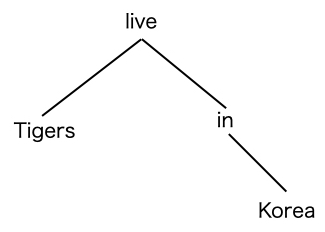
• この図で、"live"は"Tigers"の先祖、"Korea"は"in"の子孫ということが上下関係で示されている。

# 祖先の抽出
T = []
A = []

for token in doc:
    T.append(token)
    tmp = []
    for a in token.ancestors:
        tmp.append(a)
    A.append(tmp)

import pandas as pd
df_a = pd.DataFrame({"ancestors":A},index=T)
df_a

	ancestors
The	[giraffe, ate]
really	[tall, giraffe, ate]
tall	[giraffe, ate]
giraffe	[ate]
at	[giraffe, ate]
the	[zoo, at, giraffe, ate]
zoo	[at, giraffe, ate]
ate	[]
the	[leaves, ate]
green	[leaves, ate]
leaves	[ate]
off	[ate]
the	[tree, off, ate]
tree	[off, ate]
.	[ate]

# 子孫の抽出
T = []
C = []

for token in doc:
    T.append(token)
    tmp = []
    for c in token.children:
        tmp.append(c)
    C.append(tmp)

df_c = pd.DataFrame({"children":C},index=T)
df_c

	children
The	[]
really	[]
tall	[really]
giraffe	[The, tall, at]
at	[zoo]
the	[]
zoo	[the]
ate	[giraffe, leaves, off, .]
the	[]
green	[]
leaves	[the, green]
off	[tree]
the	[]
tree	[the]
.	[]

演習問題1

• 以下の文において動詞(ROOT)が直接統率している単語を"nsubj+dative+dobj+npadvmod+punct"と表現することとします。

I sent John the letter yesterday.

• これはある意味「5文型」のような文の構造を示すものになります。

• ../DATA01/sentences.txtには約1000文が含まれています。

• このデータは、文に対してその難しさを教育の「プロ」的な人がCEFRという基準に基づいて評価したものです。

• このデータのすべての文において動詞(ROOT)が直接統率している単語を上のように抽出して、pandasのデータフレームに保存し、最初の10行を降順で出力しなさい。

import pandas as pd
import matplotlib.pyplot as plt
%matplotlib inline

# 仮のデータ
D = {"A":25,"B":322,"C":66,"D":120,"E":95}

# データフレームに変換
df = pd.DataFrame.from_dict(D,orient="index",columns=["frequency"])

# 降順に並べ替え
df2 = df.sort_values(by="frequency",ascending=False)

df2.head(10)

	frequency
B	322
D	120
E	95
C	66
A	25