5.3 ニューラルネットワークを用いた分散表現の仮定
5.3.1 モデル
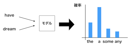
- ニューラルネットワークを用いて単語をベクトルで表すために以下のようなモデルを仮定します。
- 以下の空欄にはどのような単語が出現するでしょうか。
- I have ___ dream.
- この空欄に入る単語を予測するためにこの単語の両隣の単語のみを利用します。
- つまり、周囲の単語(コンテクスト)から単語を予測するモデルです。
- モデルを図示すると以下のようになります。
- 上の文に正解があるとした場合、これは今まで学んできたニューラルネットワークが利用できます。
- コンテクストをなんらかのベクトルで表現して、確率を出力し、正解と照らし合わせてモデルを修正することができます。
5.3.2 word2vec
- 以下のように単語をone-hotベクトルで表します。
単語|単語ID|one-hotベクトル -----|-----|----- have |1|(0,1,0,0,0)| dream |4|(0,0,0,1,0)|
- これは、語彙数と同じ数の要素を持つベクトルに単語IDの該当する箇所に1、残りを0として表現したものです。
- このようにすれば、ニューラルネットの入力層の数を固定することができます。
- 中間層を3つにした場合、以下になります。
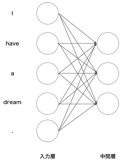
- バイアスがないモデルを設定すると入力層から中間層への変換は以下のようになります。
$$ \begin{pmatrix} t_1 & t_2 & t_3 & t_4 & t_5 \end{pmatrix} \times \begin{pmatrix} w_{11} & w_{12} & w_{13}\\ w_{21} & w_{22} & w_{23}\\ w_{31} & w_{32} & w_{33}\\ w_{41} & w_{42} & w_{43}\\ w_{51} & w_{52} & w_{53}\\ \end{pmatrix} $$
- one-hotベクトルなので、重みの行がそれぞれの計算結果になります。
- つまり、入力$(1,0,0,0,0)$の計算結果は$(w_{11},w_{12},w_{13})$に、入力$(0,1,0,0,0)$の計算結果は$(w_{21},w_{22},w_{23})$になります。
- 以下で確かめてみましょう。
In [1]:
import numpy as np

c = np.array([[1,0,0,0,0]])
W = np.random.randn(5,3)
W
Out[1]:
array([[-0.24711878, -0.30217212,  0.63086996],
       [-0.37294652, -0.84015553, -0.28290709],
       [-0.0405715 , -1.63738344,  0.236249  ],
       [ 1.76594367,  0.86563884, -0.08400158],
       [-1.56782028,  0.43182792,  0.01732045]])
In [2]:
np.dot(c,W)
Out[2]:
array([[-0.24711878, -0.30217212, 0.63086996]])
- コンテクスト(両隣の単語)である単語を予測するモデルで出力層を考えると以下のようになります。
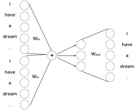
- このニューラルネットワークの重みこそがword2vecです。
- 十分に学習したニューラルネットワークの重みは、共起する単語を正確に予測します。
- 入力はone-hotベクトルなので、入力から中間層への掛け算の重みそのものがその単語の分散表現と見なすことができます。
- また、中間層から出力層への重みはその分散表現から我々が欲しい情報を抽出するプロセスと見做すことができます(中間層から出力層への重みも分散表現と見なして、入力から中間層への重みと合わせて利用する場合もあります)。
注: 元々はword2vecはパッケージの名称でしたが、この仕組み全体をword2vecと呼ぶようになりました。コンテクストからある単語を予測するモデルをContinuous Bag of Words (CBOW)と言います。
5.3.3 gensimでword2vec
- 授業で扱った方法で推論に基づく分散表現を得るためには計算時間が膨大になってしまうので、gensimというパッケージを使用します。
- word2vecで人間の実感に合う結果を得るためにはかなり大きなコーパスが必要で、
- また、かなりの計算時間を要するので、ここでは小規模なコーパスを用います。
コーパスの準備
In [3]:
from nltk import sent_tokenize, word_tokenize

text_law = open("../corpus/eng_wikipedia_2016_100K-sentences.txt","r").read()
text_sent = sent_tokenize(text_law)

text_word = []

for t in text_sent:
    text_word.append(word_tokenize(t.lower()))
../corpus/eng_news_2023_100K-sentences.txtもありますので時間があれば試してみてください。
In [4]:
# 中身の確認
print(text_word[0:2])
[['0.41', '%', 'of', 'the', 'population', 'were', 'hispanic', 'or', 'latino', 'of', 'any', 'race', '.'], ["'06", 'dtas', 'appear', 'to', 'have', 'made', 'essentially', 'simultaneous', 'and', 'duplicative', 'amendments', 'to', 'the', 'code', 'and', 'its', 'notes', '.']]
gensimの使い方
In [7]:
# word2vecのimport

from gensim.models import Word2Vec

# インスタンスの生成
model = Word2Vec(text_word,vector_size=100,window=5,min_count=5,workers=4)

# text_word: 対象の単語列
# size: 中間層の数(分散表現の次元)
# window: 周辺単語の数
# min_count: カウントする単語の最小出現数
# workers: 処理のスレッド数(とりあえず、4を引数とする)
In [8]:
# モデルの学習
model.train(text_word,total_examples=len(text_word),epochs=100)

# text_word: 対象の単語列
# total_examples: 対象の単語列の要素数
# epochs: 学習回数
Out[8]:
(161634957, 237762700)
In [9]:
# 得られた分散表現の確認
model.wv["computer"]
Out[9]:
array([-0.9481552 , -2.0022032 ,  0.25612912,  0.60312504, -0.15007946,
       -0.09309538, -2.1876633 ,  2.9426012 ,  1.5048038 , -1.1256055 ,
       -0.22765541, -0.50390947, -0.49141726, -0.74244905,  0.73845863,
       -0.91904986,  0.95638585,  0.12524813, -1.5118483 , -1.2372291 ,
        1.4795462 ,  1.491271  , -1.8316355 , -0.38170904, -3.061103  ,
        0.90220094,  1.5423411 ,  0.79568684,  1.329155  , -2.3904293 ,
       -1.7143707 ,  3.697996  , -0.4145198 ,  1.6256071 ,  1.0141512 ,
       -1.722769  , -2.660352  ,  3.7928798 ,  2.825483  ,  1.4961097 ,
       -0.66543734,  0.33961397,  0.35156596, -0.37759066,  1.1190388 ,
        0.828275  ,  0.5119422 ,  1.3980743 , -0.8327454 ,  2.3599808 ,
       -0.4315281 , -1.2972561 , -1.210235  , -1.0022051 ,  1.1044235 ,
       -1.5984268 ,  0.8530144 , -0.7984974 , -1.0899805 , -0.3103796 ,
       -3.5237415 ,  0.48103216,  0.39640257,  3.1542735 , -4.0706472 ,
       -0.7761364 , -0.8692984 ,  1.2463304 , -1.9353082 ,  1.2774323 ,
        0.55495745, -0.24177718, -1.0351473 ,  2.038302  ,  1.7747267 ,
        0.6954424 ,  0.85249096, -4.364183  , -1.4305117 , -0.12556091,
        3.19934   , -0.92910475,  0.45213526,  0.44694698,  0.16630884,
       -0.5260607 , -1.7508948 ,  1.9957045 , -1.3529396 ,  0.08757394,
        4.6617293 ,  0.11998807, -1.0198135 ,  1.8547372 ,  1.2287345 ,
        2.2353525 ,  1.7513536 ,  4.8796496 , -0.70683736,  0.21978499],
      dtype=float32)
In [10]:
# 似た意味の単語Top 10
# 0から1の値をとり、0が似ていない、1が同じ意味。

model.wv.most_similar("cat")
Out[10]:
[('protagonist', 0.4671483337879181),
 ('mother', 0.4510372281074524),
 ('judas', 0.4479161202907562),
 ('scarlet', 0.44576889276504517),
 ('steed', 0.44435206055641174),
 ('wasp', 0.4430996775627136),
 ('stark', 0.4423791170120239),
 ('muhammad', 0.441325843334198),
 ('harry', 0.44092264771461487),
 ('cock', 0.435820996761322)]
In [11]:
# 2つの単語の類似度
model.wv.similarity(w1="dog",w2="cat")
Out[11]:
np.float32(0.40256986)
In [12]:
# 2つの単語の類似度
model.wv.similarity(w1="dog",w2="pig")
Out[12]:
np.float32(0.46394616)
In [13]:
# 仲間外れを見つける
model.wv.doesnt_match(["windows","apple","banana"])
Out[13]:
'banana'
In [14]:
# 与えられたコンテクストで出現する確率が高い単語
model.predict_output_word(["apple","notebook"],topn=10)
Out[14]:
[('ii', np.float32(0.367777)),
 ('ibm', np.float32(0.09022928)),
 ('desktop', np.float32(0.036435977)),
 ('printers', np.float32(0.031823587)),
 ('portable', np.float32(0.02446387)),
 ('apple', np.float32(0.017077362)),
 ('mac', np.float32(0.016907137)),
 ('flash', np.float32(0.016028412)),
 ('iii', np.float32(0.013191687)),
 ('monopoly', np.float32(0.010018623))]
In [15]:
# JapanからTokyoを引くと
model.wv.similar_by_vector(model.wv["japan"] - model.wv["tokyo"])
Out[15]:
[('japan', 0.6632276177406311),
 ('china', 0.4878672957420349),
 ('commonwealth', 0.4340512752532959),
 ('communism', 0.4304722547531128),
 ('argentina', 0.42550596594810486),
 ('europe', 0.41875118017196655),
 ('country', 0.4099924564361572),
 ('nationalist', 0.4086264371871948),
 ('russia', 0.40824493765830994),
 ('torn', 0.40799590945243835)]